|
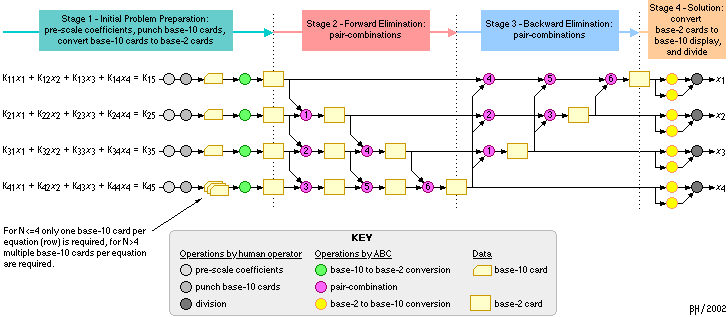
Figure 2.1: Stages of the ABC Solution Process
As exemplified for N=4 equations in 4 variables | |
|
|
The process of using the ABC to solve a set of equations can be broken into four stages. These are shown in figure 2.1, which can be seen as a practical enhancement of figure 1.2 of the Principles section. However, in figure 2.1 the backward elimination operations have been flipped about the diagonal relative to the earlier figure. The colours of the stages corresponds between the two figures.
Six types of operations are involved in these stages (see the KEY in figure 2.1), three of which do not involve the ABC, and three of which are performed by the ABC as directed by the human operator.
The ABC performs arithmetic using the binary number system, necessitating conversion between base-10 and base-2 data. Data is initially accepted into the ABC on base-10 cards. Base-2 cards are used for intermediate storage within and between stages.
|
Figure 2.1: Stages of the ABC Solution Process
As exemplified for N=4 equations in 4 variables | |
|
Stage 1 - Initial Problem Preparation: The initial coefficients are pre-scaled, punched onto base-10 cards and, using the ABC, converted to base-2.
The ABC deals with integer numbers, so to obtain some resolution in the results the coefficients likely need to be pre-scaled. The entire set of equations is multiplied by some factor such as 1,000,000. While it may seem desirable to scale the coefficients up to the most-significant-digits of the machine (10^14...10^15), scaling up too far may result in overflow during pair-combinations later.
Pre-scaling may also be used to get around a shortcoming of the ABC. In contrast to more complete division algorithms, the ABC does not shift the divisor up to match the magnitude of the dividend. Consequently, if the difference in magnitude of two coefficients being eliminated is large the solution time may become prohibitive. For example, a pair-combination in which the coefficient to be eliminated is 1 from 10000 will result in the ABC requiring 10000 revolutions - more than 2 hours - for a single pair combination. A more tailored approach to pre-scaling, in which the equations are scaled by different factors, may be able to shorten the solution time.
The pre-scaled coefficients are punched onto base-10 cards. Each base-10 card can hold up to 5 coefficients so for N<=4 one card per equation suffices. For 5<=N<=29 up to six base-10 cards per equation are required.
The ABC is then used to convert the coefficients on the base-10 cards to base-2, and punch them out on base-2 cards, one card for each initial equation.
Stage 2 - Forward Elimination: The ABC is used to perform pair-combinations. Additional base-2 cards are produced.
Stage 3 - Backward Elimination: The ABC is used to perform more pair-combinations. Note that while the pair-combination operation used in stages 2 and 3 is identical, the dataflow is different for the two stages.
The pair-combinations of stages 2 and 3 can be performed in either a row-by-row or column-by-column sequence. Indicated in figure 2.1 is the suggested choice of column-by-column for stage 2 and row-by-row for stage 3. For stage 2 a column-by-column sequence provides some efficiencies in card loading and machine setup. For stage 3 using a row-by-row sequence makes it possible to eliminate the punching and reading of cards internal to the stage.
Stage 4 - Solution: The ABC is used to convert the final set of N equations in one variable from base-2 to base-10. This requires two conversions for each equation, the result of each conversion is displayed on the base-10 display of the ABC. The two conversions for each equation are divided (with a desk calculator or manually) to finally obtain the value of each variable.
Card Management: Keeping track of the cards and one's place in the process can become difficult for even small N. Perhaps the nicest scheme to organise this is to have an N by N array of bins beside the ABC into which cards can be placed in a manner which follows the descending columns of cards in figure 2.1. A glance at the bins gives an indication of the state of the process. The downside to this scheme is the space the bins would occupy as N becomes large. Other schemes could reduce the array to 2 or 3 columns by N rows and involve the use of some form of marker placed on or over the cards.
|
1. Principles
| 2. Stages
| 3. Equipment
| 4. Flowchart
Proof-of-Concept | Architecture | ASM | Manual | Simulation ABC |
bhilpert 2002 |